Introduction to Computer Vision: Plant Seedlings Classification
Project by Noor Aftab
Problem Statement
Context
In recent times, the field of agriculture has been in urgent need of modernizing, since the amount of manual work people need to put in to check if plants are growing correctly is still highly extensive. Despite several advances in agricultural technology, people working in the agricultural industry still need to have the ability to sort and recognize different plants and weeds, which takes a lot of time and effort in the long term. The potential is ripe for this trillion-dollar industry to be greatly impacted by technological innovations that cut down on the requirement for manual labor, and this is where Artificial Intelligence can actually benefit the workers in this field, as the time and energy required to identify plant seedlings will be greatly shortened by the use of AI and Deep Learning. The ability to do so far more efficiently and even more effectively than experienced manual labor, could lead to better crop yields, the freeing up of human inolvement for higher-order agricultural decision making, and in the long term will result in more sustainable environmental practices in agriculture as well.
Objective
The aim of this project is to Build a Convolutional Neural Netowrk to classify plant seedlings into their respective categories.
Data Dictionary
The Aarhus University Signal Processing group, in collaboration with the University of Southern Denmark, has recently released a dataset containing images of unique plants belonging to 12 different species.
The data file names are:
- images.npy
- Label.csv
Due to the large volume of data, the images were converted to the images.npy file and the labels are also put into Labels.csv, so that we can work on the data/project seamlessly without having to worry about the high data volume.
The goal of the project is to create a classifier capable of determining a plant’s species from an image.
List of Species
- Black-grass
- Charlock
- Cleavers
- Common Chickweed
- Common Wheat
- Fat Hen
- Loose Silky-bent
- Maize
- Scentless Mayweed
- Shepherds Purse
- Small-flowered Cranesbill
- Sugar beet
Importing Libraries
In [ ]:import os #Libraries to manipulate dataimport numpy as np import pandas as pd #Libraries to visualize dataimport matplotlib.pyplot as plt import math import cv2 import seaborn as sns #Tensorflow modulesimport tensorflow as tf from tensorflow.keras.preprocessing.image import ImageDataGenerator from tensorflow.keras.models import Sequential from tensorflow.keras.layers import Dense, Dropout, Flatten, Conv2D, MaxPooling2D, BatchNormalization from tensorflow.keras.optimizers import Adam, SGD from sklearn import preprocessing from sklearn import metrics from sklearn.model_selection import train_test_split from sklearn.metrics import confusion_matrix from sklearn.preprocessing import LabelBinarizer #Display images using OpenCVfrom google.colab.patches import cv2_imshow from sklearn.model_selection import train_test_split from tensorflow.keras import backend from keras.callbacks import ReduceLROnPlateau import random from tensorflow.keras.callbacks import ReduceLROnPlateau import warnings warnings.filterwarnings(‘ignore’)
Load the dataset
In [ ]:from google.colab import drive drive.mount(‘/content/drive’) Drive already mounted at /content/drive; to attempt to forcibly remount, call drive.mount(“/content/drive”, force_remount=True).
Loading images and labels
In [ ]:#load images file of dataset. Since images is npy, we will use np.load() images = np.load(‘/content/drive/MyDrive/Plant_Classification/images.npy’) #load label files of dataset labels = pd.read_csv(‘/content/drive/MyDrive/Plant_Classification/Labels.csv’)
Data Overview
Understand the shape of the dataset
In [ ]:#printing the shape of images and labels print(“Images: “,images.shape) print(“Labels:”, labels.shape) Images: (4750, 128, 128, 3) Labels: (4750, 1)
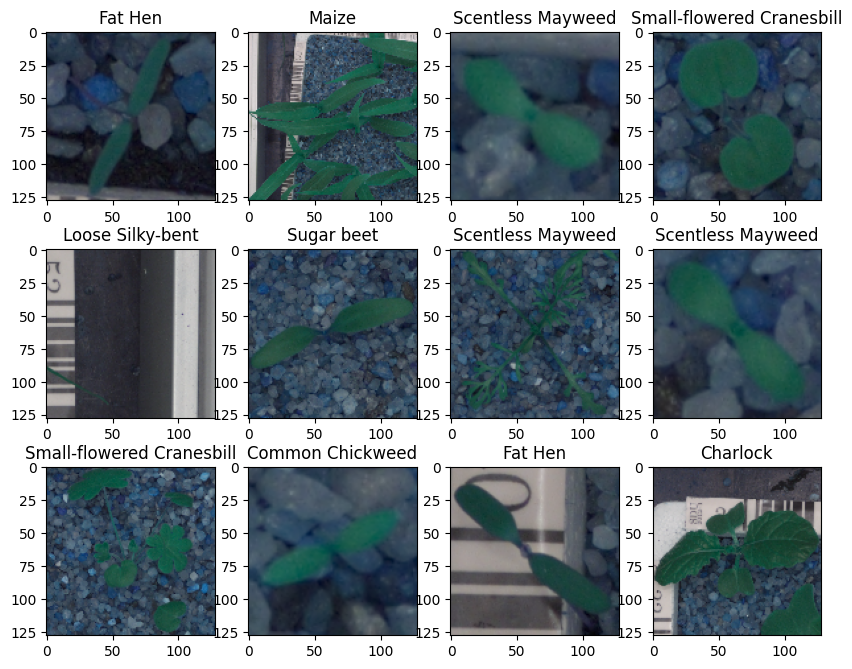
Plotting random Images from our dataset
In [ ]:#Defining a function to visualize few images from the dataset.def plot_images(images, labels): # Define the number of classes num_classes = 10 # Get unique categories categories = np.unique(labels) # Create a dictionary ‘keys’ from the ‘Label’ column in the DataFrame ‘labels’ keys = dict(labels[‘Label’]) # Creating a 3×4 grid of images rows = 3 cols = 4 # Create a new figure with a specified size (10 inches wide and 8 inches tall) fig = plt.figure(figsize=(10, 8)) # Loop to display images in a gridfor i in range(cols): for j in range(rows): # Generate a random index within the range of the number of labels random_index = np.random.randint(0, len(labels)) # Add a subplot to the figure, with ‘rows’ rows and ‘cols’ columns ax = fig.add_subplot(rows, cols, i * rows + j + 1) # Display the image at the random_index position in the ‘images’ array ax.imshow(images[random_index, :]) # Displaying the title of each image using the label from the ‘keys’ dictionary ax.set_title(keys[random_index]) # Show the entire figure with the grid of images plt.show()
In [ ]:#Code to input the images and labels to the function and plot the images with their labels plot_images(images,labels)
Checking for Imbalanced Dataset
In [ ]:#Checking for distribution of classes in the dataset to check of imbalnced data# Calculate the counts of each category for the plot category_counts = labels[‘Label’].value_counts() # Calculate the percentage of each category category_percentage = category_counts / category_counts.sum() * 100 # Setting the default figure size for the plots to 10×7 inches for better readability plt.rcParams[“figure.figsize”] = (15,7) # Create a count plot with Seaborn ax = sns.countplot(x=‘Label’, data=labels, order=category_counts.index, palette=‘Greens_r’) # Labeling the x-axis as ‘Plant Categories’ plt.xlabel(‘Plant Categories’) # Rotating the x-axis labels by 90 degrees to prevent overlapping and improve readability plt.xticks(rotation=90) # Annotating the percentage of each category above the barsfor i, p in enumerate(ax.patches): # Calculate the height to place the annotation correctly height = p.get_height() # Adding text annotation and formatting to show up to two decimal places ax.text(p.get_x() + p.get_width()/2., height + 3, ‘{:1.2f}%’.format(category_percentage[i]), ha=“center”) # Displaying the plot plt.show()
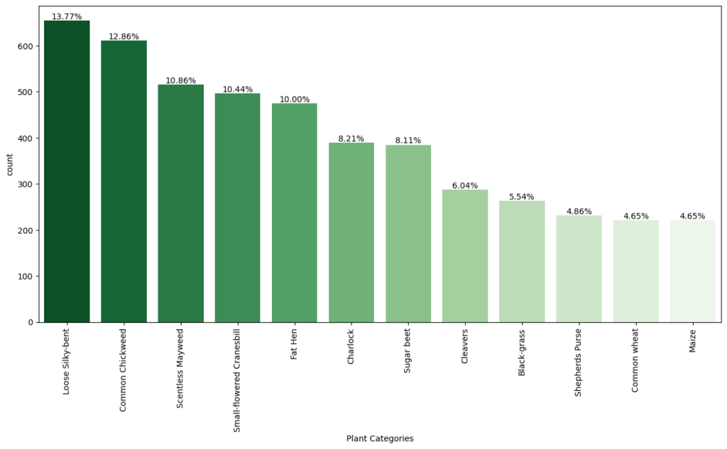
Observations
- From the chart, we can see that the classes are not evenly distributed. The class with the lowest representation (4.65% for three classes: Black-grass, Shepherd’s Purse, and Maize) could potentially be more challenging for the models to learn due to fewer training examples.
- On the other hand, Loose Silky-bent has the highest representation at 13.77%, which might mean the model will perform better on this class simply due to more training data.
Converting the images from BGR To RGB
In [ ]:#converting all images from Blue-Green-Red to Red-Green-Blue formatfor i in range(len(images)): images[i] = cv2.cvtColor(images[i], cv2.COLOR_BGR2RGB)
Reducing the size of images
In [ ]:#As the size of the images is large, it may be computationally expensive to train on these larger images.#Therefore, it is preferable to reduce the image size from 128 to 64.#creating a new array to hold the images with updated dimension of 64 x 64 images_decreased=[] height = 64 # Code to define the height as 64 width = 64 # Code to define the width as 64 dimensions = (width, height) for i in range(len(images)): images_decreased.append( cv2.resize(images[i], dimensions, interpolation=cv2.INTER_LINEAR))
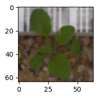
Image before resizing
In [ ]:plt.imshow(images[3])
Out[ ]:<matplotlib.image.AxesImage at 0x78f7bd9c68f0>
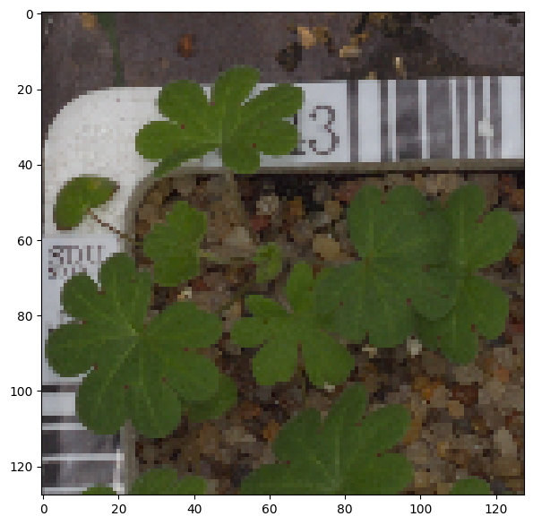
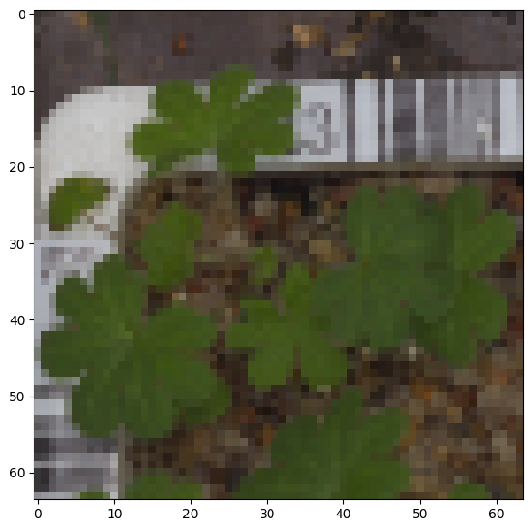
Image after resizing
In [ ]:plt.imshow(images_decreased[3])
Out[ ]:<matplotlib.image.AxesImage at 0x78f7b79bb220>
Data Preparation for Modeling
- As we have less images in our dataset, we will only use 10% of our data for testing, 10% of our data for validation and 80% of our data for training.
- We are using the train_test_split() function from scikit-learn. Here, we split the dataset into three parts, train,test and validation.
In [ ]:from sklearn.model_selection import train_test_split # Split the data into a temporary set and a test set X_temp, X_test, y_temp, y_test = train_test_split(np.array(images_decreased), labels, test_size=0.1, random_state=42, stratify=labels) # Split the temporary set into a training set and a validation set X_train, X_val, y_train, y_val = train_test_split(X_temp, y_temp, test_size=0.1, random_state=42, stratify=y_temp)
In [ ]:print(X_train.shape, y_train.shape) # Check the shape of the training data and labels print(X_val.shape, y_val.shape) # Check the shape of the validation data and labels print(X_test.shape, y_test.shape) # Check the shape of the test data and labels (3847, 64, 64, 3) (3847, 1) (428, 64, 64, 3) (428, 1) (475, 64, 64, 3) (475, 1)
Encoding the categorical data using Label Binarizer
In [ ]:#LabelBinarizer helps translate categories or labelsfrom sklearn.preprocessing import LabelBinarizer # Initialize the LabelBinarizer enc = LabelBinarizer() # Fit and transform y_train y_train_encoded = enc.fit_transform(y_train) # Transform y_val y_val_encoded = enc.transform(y_val) # Transform y_test y_test_encoded = enc.transform(y_test)
In [ ]:#checking the shape of target variables post encoding y_train_encoded.shape, y_val_encoded.shape, y_test_encoded.shape
Out[ ]:((3847, 12), (428, 12), (475, 12))
Data Normalization
Since the image pixel values range from 0-255, our method of normalization here will be scaling.
- We are dividing all the pixel values by 255 to standardize the images to have values between 0-1.
In [ ]:#Code to normalize the image pixels of train, test and validation data X_train_normalized = X_train.astype(‘float32’) / 255.0 X_val_normalized = X_val.astype(‘float32’) / 255.0 X_test_normalized = X_test.astype(‘float32’) / 255.0
Model Building
We are creating a base model using 3 pairs of Convolution and Pooling Layers.
- Next we are using the Flatten()
- We follow this with fully connected layers of 16 neurons, followed by drop out layer.
- Finally, we add the output layer using softmax activation and Adam optimizer.
In [ ]:#Clearing the backend backend.clear_session()
In [ ]:# Fixing the seed for random number generators np.random.seed(42) random.seed(42) tf.random.set_seed(42)
In [ ]:#initalize the model model1 = Sequential() #Feature Extraction#First layer with 128 neurons, relu activaiton, same padding to keep the input and output same model1.add(Conv2D(128,(3,3), activation=‘relu’, padding=‘same’, input_shape=(64, 64, 3))) #Adding Max Pooling to reduce dimension model1.add(MaxPooling2D((2,2), padding=‘same’)) #Code to create two similar convolution and max-pooling layers activation = relu model1.add(Conv2D(64,(3,3), activation=‘relu’, padding=‘same’)) model1.add(MaxPooling2D((2,2), padding=‘same’)) model1.add(Conv2D(32,(3,3), activation=‘relu’, padding=‘same’)) model1.add(MaxPooling2D((2,2), padding=‘same’)) #Flattening the output after convolution and max pooling model1.add(Flatten()) #Code to add a fully connected dense layer with 16 neurons model1.add(Dense(16,activation=‘relu’)) model1.add(Dropout(0.3)) #Code to add the output layer with 12 neurons and activation functions as softmax since this is a multi-class classification problem model1.add(Dense(12,activation=‘softmax’)) #Using Adam Optimizer opt = Adam() #Compile the model model1.compile(optimizer=opt, loss=‘categorical_crossentropy’, metrics=[‘accuracy’]) #Generate model summary model1.summary() Model: “sequential” _________________________________________________________________ Layer (type) Output Shape Param # ================================================================= conv2d (Conv2D) (None, 64, 64, 128) 3584 max_pooling2d (MaxPooling2 (None, 32, 32, 128) 0 D) conv2d_1 (Conv2D) (None, 32, 32, 64) 73792 max_pooling2d_1 (MaxPoolin (None, 16, 16, 64) 0 g2D) conv2d_2 (Conv2D) (None, 16, 16, 32) 18464 max_pooling2d_2 (MaxPoolin (None, 8, 8, 32) 0 g2D) flatten (Flatten) (None, 2048) 0 dense (Dense) (None, 16) 32784 dropout (Dropout) (None, 16) 0 dense_1 (Dense) (None, 12) 204 ================================================================= Total params: 128828 (503.23 KB) Trainable params: 128828 (503.23 KB) Non-trainable params: 0 (0.00 Byte) _________________________________________________________________
Fitting the model on train data
In [ ]:#Fitting the model on train and also using the validation data for validation history_1 = model1.fit(X_train_normalized, y_train_encoded, epochs =30, validation_data=(X_val_normalized,y_val_encoded), batch_size =32, verbose=2)
Epoch 1/30 121/121 – 3s – loss: 2.4543 – accuracy: 0.1053 – val_loss: 2.4388 – val_accuracy: 0.1379 – 3s/epoch – 24ms/step Epoch 2/30 121/121 – 1s – loss: 2.3920 – accuracy: 0.1643 – val_loss: 2.1059 – val_accuracy: 0.3575 – 1s/epoch – 9ms/step Epoch 3/30 121/121 – 1s – loss: 2.0629 – accuracy: 0.3067 – val_loss: 1.8427 – val_accuracy: 0.3925 – 1s/epoch – 9ms/step Epoch 4/30 121/121 – 1s – loss: 1.9083 – accuracy: 0.3361 – val_loss: 1.7196 – val_accuracy: 0.4252 – 1s/epoch – 9ms/step Epoch 5/30 121/121 – 1s – loss: 1.7649 – accuracy: 0.3767 – val_loss: 1.5800 – val_accuracy: 0.4720 – 1s/epoch – 10ms/step Epoch 6/30 121/121 – 1s – loss: 1.6525 – accuracy: 0.4068 – val_loss: 1.4383 – val_accuracy: 0.5350 – 1s/epoch – 9ms/step Epoch 7/30 121/121 – 1s – loss: 1.5677 – accuracy: 0.4307 – val_loss: 1.3422 – val_accuracy: 0.5327 – 1s/epoch – 9ms/step Epoch 8/30 121/121 – 1s – loss: 1.4942 – accuracy: 0.4562 – val_loss: 1.2520 – val_accuracy: 0.5654 – 1s/epoch – 9ms/step Epoch 9/30 121/121 – 1s – loss: 1.4390 – accuracy: 0.4799 – val_loss: 1.1876 – val_accuracy: 0.6051 – 1s/epoch – 9ms/step Epoch 10/30 121/121 – 1s – loss: 1.3807 – accuracy: 0.5035 – val_loss: 1.2670 – val_accuracy: 0.5794 – 1s/epoch – 9ms/step Epoch 11/30 121/121 – 1s – loss: 1.3182 – accuracy: 0.5201 – val_loss: 1.1684 – val_accuracy: 0.6168 – 1s/epoch – 9ms/step Epoch 12/30 121/121 – 1s – loss: 1.3135 – accuracy: 0.5235 – val_loss: 1.0868 – val_accuracy: 0.6355 – 1s/epoch – 9ms/step Epoch 13/30 121/121 – 1s – loss: 1.2812 – accuracy: 0.5295 – val_loss: 1.1118 – val_accuracy: 0.6285 – 1s/epoch – 9ms/step Epoch 14/30 121/121 – 1s – loss: 1.2376 – accuracy: 0.5472 – val_loss: 1.0302 – val_accuracy: 0.6449 – 1s/epoch – 10ms/step Epoch 15/30 121/121 – 1s – loss: 1.2220 – accuracy: 0.5513 – val_loss: 1.0038 – val_accuracy: 0.6869 – 1s/epoch – 9ms/step Epoch 16/30 121/121 – 1s – loss: 1.2179 – accuracy: 0.5558 – val_loss: 1.0013 – val_accuracy: 0.6846 – 1s/epoch – 9ms/step Epoch 17/30 121/121 – 1s – loss: 1.1841 – accuracy: 0.5638 – val_loss: 0.9745 – val_accuracy: 0.6893 – 1s/epoch – 10ms/step Epoch 18/30 121/121 – 1s – loss: 1.1281 – accuracy: 0.5854 – val_loss: 0.9683 – val_accuracy: 0.6893 – 1s/epoch – 10ms/step Epoch 19/30 121/121 – 1s – loss: 1.1101 – accuracy: 0.5896 – val_loss: 0.9784 – val_accuracy: 0.6659 – 1s/epoch – 10ms/step Epoch 20/30 121/121 – 1s – loss: 1.0669 – accuracy: 0.6093 – val_loss: 0.9875 – val_accuracy: 0.7033 – 1s/epoch – 10ms/step Epoch 21/30 121/121 – 1s – loss: 1.0897 – accuracy: 0.6049 – val_loss: 0.9850 – val_accuracy: 0.6846 – 1s/epoch – 10ms/step Epoch 22/30 121/121 – 1s – loss: 1.0730 – accuracy: 0.6044 – val_loss: 0.9444 – val_accuracy: 0.7009 – 1s/epoch – 10ms/step Epoch 23/30 121/121 – 1s – loss: 1.0391 – accuracy: 0.6174 – val_loss: 0.9757 – val_accuracy: 0.7126 – 1s/epoch – 10ms/step Epoch 24/30 121/121 – 1s – loss: 1.0300 – accuracy: 0.6220 – val_loss: 0.9271 – val_accuracy: 0.6986 – 1s/epoch – 10ms/step Epoch 25/30 121/121 – 1s – loss: 1.0076 – accuracy: 0.6309 – val_loss: 0.9220 – val_accuracy: 0.7126 – 1s/epoch – 10ms/step Epoch 26/30 121/121 – 1s – loss: 0.9627 – accuracy: 0.6444 – val_loss: 0.8981 – val_accuracy: 0.7150 – 1s/epoch – 10ms/step Epoch 27/30 121/121 – 1s – loss: 0.9734 – accuracy: 0.6348 – val_loss: 0.9724 – val_accuracy: 0.7056 – 1s/epoch – 9ms/step Epoch 28/30 121/121 – 1s – loss: 0.9421 – accuracy: 0.6543 – val_loss: 0.9244 – val_accuracy: 0.7243 – 1s/epoch – 9ms/step Epoch 29/30 121/121 – 1s – loss: 0.9490 – accuracy: 0.6501 – val_loss: 0.9061 – val_accuracy: 0.7056 – 1s/epoch – 10ms/step Epoch 30/30 121/121 – 1s – loss: 0.9277 – accuracy: 0.6631 – val_loss: 0.8989 – val_accuracy: 0.7173 – 1s/epoch – 9ms/step
Model Evaluation
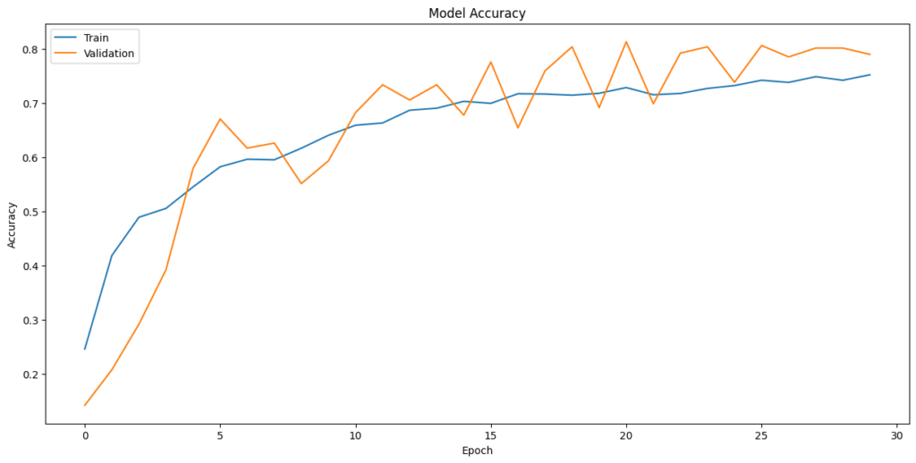
In [ ]:plt.plot(history_1.history[‘accuracy’]) plt.plot(history_1.history[‘val_accuracy’]) plt.title(‘Model Accuracy’) plt.ylabel(‘Accuracy’) plt.xlabel(‘Epochs’) plt.legend([‘Train’,’Validation’],loc=‘upper left’) plt.show()

Observations:
- The fluctuating validation loss and accuracy, especially towards the end of training, are indicative of potential overfitting
- Training Time: The model trains relatively quickly, with each epoch taking around 1-2 seconds, which is a positive aspect.
- Final Validation Accuracy: The final validation accuracy around 0.6631 suggests that the model achieves reasonable performance on the validation data, but there may still be room for improvement.
Evaluate the model on test data
In [ ]:# X_test_normalized: The normalized test feature data# y_test_encoded: The encoded test target labels# verbose=2: Display evaluation results accuracy = model1.evaluate(X_test_normalized, y_test_encoded, verbose=2) 15/15 – 0s – loss: 1.0660 – accuracy: 0.6611 – 86ms/epoch – 6ms/step
In [ ]:# Here we would get the output as probablities for each category y_pred = model1.predict(X_test_normalized) 15/15 [==============================] – 0s 3ms/step
Observations
- The overall accuracy of the model is 0.6611, which suggests that it correctly predicts the plant species approximately 66.11% of the time on the test set.
- The classes are not equally easy or difficult for the model to predict. Some classes have higher precision and recall, while others have lower values, indicating variability in the model’s performance across different species.
Plotting the Confusion Matrix
In [ ]:# Obtain categorical variables from y_test_encoded and y_pred y_pred_arg = np.argmax(y_pred, axis=1) y_test_arg = np.argmax(y_test_encoded, axis=1) # Plotting confusion matrix with ‘viridis’ cmap (green color map) confusion_matrix = tf.math.confusion_matrix(y_test_arg, y_pred_arg) f, ax = plt.subplots(figsize=(12, 12)) sns.heatmap( confusion_matrix, annot=True, linewidths=0.4, fmt=‘d’, square=True, ax=ax, cmap=‘Greens’ # Set the colormap to Green ) # Setting labels to both axes ax.set_xlabel(‘Predicted labels’) ax.set_ylabel(‘True labels’) ax.set_title(‘Confusion Matrix’) ax.xaxis.set_ticklabels(list(enc.classes_), rotation=40) ax.yaxis.set_ticklabels(list(enc.classes_), rotation=20) plt.show()
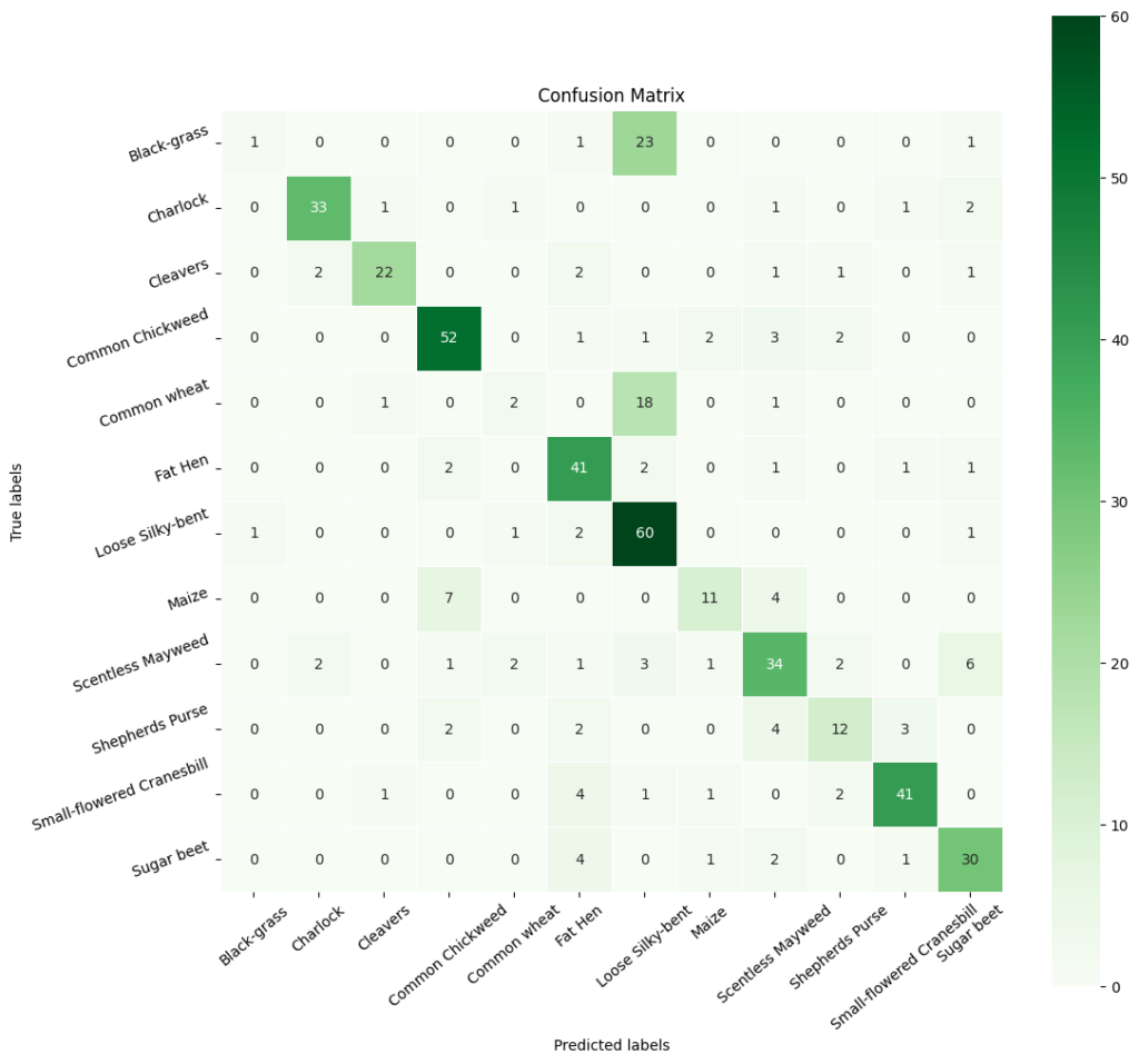
In [ ]:# Calculate the classification report cr1 = metrics.classification_report(y_test_arg, y_pred_arg) # Print the classification report print(cr1) precision recall f1-score support 0 0.50 0.04 0.07 26 1 0.89 0.85 0.87 39 2 0.88 0.76 0.81 29 3 0.81 0.85 0.83 61 4 0.33 0.09 0.14 22 5 0.71 0.85 0.77 48 6 0.56 0.92 0.69 65 7 0.69 0.50 0.58 22 8 0.67 0.65 0.66 52 9 0.63 0.52 0.57 23 10 0.87 0.82 0.85 50 11 0.71 0.79 0.75 38 accuracy 0.71 475 macro avg 0.69 0.64 0.63 475 weighted avg 0.71 0.71 0.69 475
Model Performance Improvement
Reducing the Learning Rate:
ReduceLRonPlateau() is a function that will be used to decrease the learning rate by some factor, if the loss is not decreasing for some time. This may start decreasing the loss at a smaller learning rate. There is a possibility that the loss may still not decrease. This may lead to executing the learning rate reduction again in an attempt to achieve a lower loss.
In [ ]:# Code to monitor val_accuracy learning_rate_reduction = ReduceLROnPlateau(monitor=‘val_accuracy’, patience=3, verbose=1, factor=0.5, min_lr=0.00001)
Data Augmentation
In [ ]:#Clear Backendfrom tensorflow.keras import backend backend.clear_session() #fixing random seed generatorsimport random np.random.seed(42) random.seed(42) tf.random.set_seed(42)
In [ ]:#Code to set the rotation_range to 20 train_datagen = ImageDataGenerator( rotation_range=20, # Set the rotation range to 20 degrees fill_mode=‘nearest’ )
In [ ]:# Intializing a sequential model model2 = Sequential() # Code to add the first conv layer with 64 filters and kernel size 3×3 , padding ‘same’ provides the output size same as the input size# Input_shape denotes input image dimension images model2.add(Conv2D(64, (3,3), activation=‘relu’, padding=“same”, input_shape=(64, 64, 3))) # Code to add max pooling to reduce the size of output of first conv layer model2.add(MaxPooling2D((2, 2), padding = ‘same’)) model2.add(Conv2D(32, (3, 3), activation=‘relu’, padding=“same”)) model2.add(MaxPooling2D((2, 2), padding = ‘same’)) model2.add(BatchNormalization()) # flattening the output of the conv layer after max pooling to make it ready for creating dense connections model2.add(Flatten()) # Adding a fully connected dense layer with 16 neurons model2.add(Dense(16, activation=‘relu’)) # Code to add dropout with dropout_rate=0.3 model2.add(Dropout(0.3)) # Adding the output layer with 12 neurons and activation functions as softmax since this is a multi-class classification problem model2.add(Dense(12, activation=‘softmax’)) # Initializing Adam Optimimzer opt=Adam() # Compiling model model2.compile(optimizer=opt, loss=‘categorical_crossentropy’, metrics=[‘accuracy’]) # Generating the summary of the model model2.summary() Model: “sequential” _________________________________________________________________ Layer (type) Output Shape Param # ================================================================= conv2d (Conv2D) (None, 64, 64, 64) 1792 max_pooling2d (MaxPooling2 (None, 32, 32, 64) 0 D) conv2d_1 (Conv2D) (None, 32, 32, 32) 18464 max_pooling2d_1 (MaxPoolin (None, 16, 16, 32) 0 g2D) batch_normalization (Batch (None, 16, 16, 32) 128 Normalization) flatten (Flatten) (None, 8192) 0 dense (Dense) (None, 16) 131088 dropout (Dropout) (None, 16) 0 dense_1 (Dense) (None, 12) 204 ================================================================= Total params: 151676 (592.48 KB) Trainable params: 151612 (592.23 KB) Non-trainable params: 64 (256.00 Byte) _________________________________________________________________
In [ ]:# Set the number of epochs and batch size epochs =30 batch_size=64 # Fit the model using the ImageDataGenerator with data augmentation history_2 = model2.fit(train_datagen.flow(X_train_normalized, y_train_encoded, batch_size=batch_size, shuffle=False), epochs=epochs, steps_per_epoch= X_train_normalized.shape[0] //batch_size, validation_data=(X_val_normalized, y_val_encoded), verbose=1, callbacks=[learning_rate_reduction] ) Epoch 1/30 60/60 [==============================] – 6s 73ms/step – loss: 2.1460 – accuracy: 0.2464 – val_loss: 2.4110 – val_accuracy: 0.1425 – lr: 0.0010 Epoch 2/30 60/60 [==============================] – 4s 72ms/step – loss: 1.6699 – accuracy: 0.4187 – val_loss: 2.2931 – val_accuracy: 0.2079 – lr: 0.0010 Epoch 3/30 60/60 [==============================] – 4s 72ms/step – loss: 1.4746 – accuracy: 0.4893 – val_loss: 2.1898 – val_accuracy: 0.2921 – lr: 0.0010 Epoch 4/30 60/60 [==============================] – 4s 74ms/step – loss: 1.4168 – accuracy: 0.5057 – val_loss: 2.0589 – val_accuracy: 0.3925 – lr: 0.0010 Epoch 5/30 60/60 [==============================] – 4s 74ms/step – loss: 1.2908 – accuracy: 0.5453 – val_loss: 1.8826 – val_accuracy: 0.5794 – lr: 0.0010 Epoch 6/30 60/60 [==============================] – 4s 71ms/step – loss: 1.1815 – accuracy: 0.5823 – val_loss: 1.6619 – val_accuracy: 0.6706 – lr: 0.0010 Epoch 7/30 60/60 [==============================] – 4s 71ms/step – loss: 1.1701 – accuracy: 0.5964 – val_loss: 1.5149 – val_accuracy: 0.6168 – lr: 0.0010 Epoch 8/30 60/60 [==============================] – 4s 70ms/step – loss: 1.1466 – accuracy: 0.5953 – val_loss: 1.3013 – val_accuracy: 0.6262 – lr: 0.0010 Epoch 9/30 60/60 [==============================] – ETA: 0s – loss: 1.0864 – accuracy: 0.6167 Epoch 9: ReduceLROnPlateau reducing learning rate to 0.0005000000237487257. 60/60 [==============================] – 4s 70ms/step – loss: 1.0864 – accuracy: 0.6167 – val_loss: 1.3709 – val_accuracy: 0.5514 – lr: 0.0010 Epoch 10/30 60/60 [==============================] – 4s 72ms/step – loss: 0.9963 – accuracy: 0.6405 – val_loss: 1.2891 – val_accuracy: 0.5935 – lr: 5.0000e-04 Epoch 11/30 60/60 [==============================] – 4s 70ms/step – loss: 0.9561 – accuracy: 0.6590 – val_loss: 1.0101 – val_accuracy: 0.6822 – lr: 5.0000e-04 Epoch 12/30 60/60 [==============================] – 4s 71ms/step – loss: 0.9293 – accuracy: 0.6632 – val_loss: 0.8704 – val_accuracy: 0.7336 – lr: 5.0000e-04 Epoch 13/30 60/60 [==============================] – 5s 78ms/step – loss: 0.8915 – accuracy: 0.6868 – val_loss: 0.9048 – val_accuracy: 0.7056 – lr: 5.0000e-04 Epoch 14/30 60/60 [==============================] – 5s 77ms/step – loss: 0.8654 – accuracy: 0.6905 – val_loss: 0.9051 – val_accuracy: 0.7336 – lr: 5.0000e-04 Epoch 15/30 60/60 [==============================] – ETA: 0s – loss: 0.8497 – accuracy: 0.7031 Epoch 15: ReduceLROnPlateau reducing learning rate to 0.0002500000118743628. 60/60 [==============================] – 5s 76ms/step – loss: 0.8497 – accuracy: 0.7031 – val_loss: 1.0092 – val_accuracy: 0.6776 – lr: 5.0000e-04 Epoch 16/30 60/60 [==============================] – 4s 74ms/step – loss: 0.8292 – accuracy: 0.6994 – val_loss: 0.7460 – val_accuracy: 0.7757 – lr: 2.5000e-04 Epoch 17/30 60/60 [==============================] – 4s 71ms/step – loss: 0.7911 – accuracy: 0.7172 – val_loss: 1.1533 – val_accuracy: 0.6542 – lr: 2.5000e-04 Epoch 18/30 60/60 [==============================] – 4s 72ms/step – loss: 0.7830 – accuracy: 0.7166 – val_loss: 0.8083 – val_accuracy: 0.7593 – lr: 2.5000e-04 Epoch 19/30 60/60 [==============================] – 4s 71ms/step – loss: 0.7788 – accuracy: 0.7145 – val_loss: 0.7060 – val_accuracy: 0.8037 – lr: 2.5000e-04 Epoch 20/30 60/60 [==============================] – 4s 72ms/step – loss: 0.7684 – accuracy: 0.7179 – val_loss: 0.9217 – val_accuracy: 0.6916 – lr: 2.5000e-04 Epoch 21/30 60/60 [==============================] – 4s 75ms/step – loss: 0.7539 – accuracy: 0.7285 – val_loss: 0.6886 – val_accuracy: 0.8131 – lr: 2.5000e-04 Epoch 22/30 60/60 [==============================] – 4s 70ms/step – loss: 0.7550 – accuracy: 0.7153 – val_loss: 0.9083 – val_accuracy: 0.6986 – lr: 2.5000e-04 Epoch 23/30 60/60 [==============================] – 4s 72ms/step – loss: 0.7723 – accuracy: 0.7177 – val_loss: 0.7199 – val_accuracy: 0.7921 – lr: 2.5000e-04 Epoch 24/30 60/60 [==============================] – ETA: 0s – loss: 0.7410 – accuracy: 0.7269 Epoch 24: ReduceLROnPlateau reducing learning rate to 0.0001250000059371814. 60/60 [==============================] – 4s 70ms/step – loss: 0.7410 – accuracy: 0.7269 – val_loss: 0.7285 – val_accuracy: 0.8037 – lr: 2.5000e-04 Epoch 25/30 60/60 [==============================] – 4s 70ms/step – loss: 0.7417 – accuracy: 0.7322 – val_loss: 0.8511 – val_accuracy: 0.7383 – lr: 1.2500e-04 Epoch 26/30 60/60 [==============================] – 4s 71ms/step – loss: 0.7136 – accuracy: 0.7420 – val_loss: 0.6797 – val_accuracy: 0.8061 – lr: 1.2500e-04 Epoch 27/30 60/60 [==============================] – ETA: 0s – loss: 0.7221 – accuracy: 0.7380 Epoch 27: ReduceLROnPlateau reducing learning rate to 6.25000029685907e-05. 60/60 [==============================] – 4s 70ms/step – loss: 0.7221 – accuracy: 0.7380 – val_loss: 0.7485 – val_accuracy: 0.7850 – lr: 1.2500e-04 Epoch 28/30 60/60 [==============================] – 4s 72ms/step – loss: 0.6899 – accuracy: 0.7486 – val_loss: 0.6873 – val_accuracy: 0.8014 – lr: 6.2500e-05 Epoch 29/30 60/60 [==============================] – 4s 74ms/step – loss: 0.7054 – accuracy: 0.7420 – val_loss: 0.7191 – val_accuracy: 0.8014 – lr: 6.2500e-05 Epoch 30/30 60/60 [==============================] – ETA: 0s – loss: 0.6911 – accuracy: 0.7520 Epoch 30: ReduceLROnPlateau reducing learning rate to 3.125000148429535e-05. 60/60 [==============================] – 4s 73ms/step – loss: 0.6911 – accuracy: 0.7520 – val_loss: 0.7066 – val_accuracy: 0.7897 – lr: 6.2500e-05
Model Evaluation
In [ ]:plt.plot(history_2.history[‘accuracy’]) plt.plot(history_2.history[‘val_accuracy’]) plt.title(‘Model Accuracy’) plt.ylabel(‘Accuracy’) plt.xlabel(‘Epoch’) plt.legend([‘Train’,’Validation’], loc=‘upper left’) plt.show()
Evaluate the model on test data
In [ ]:#Code to evaluate the model on test data accuracy = model2.evaluate(X_test_normalized, y_test_encoded, verbose=2) 15/15 – 0s – loss: 0.8112 – accuracy: 0.7537 – 68ms/epoch – 5ms/step
In [ ]:#Code to obtain the output probabilities y2_pred = model2.predict(X_test_normalized) 15/15 [==============================] – 0s 2ms/step
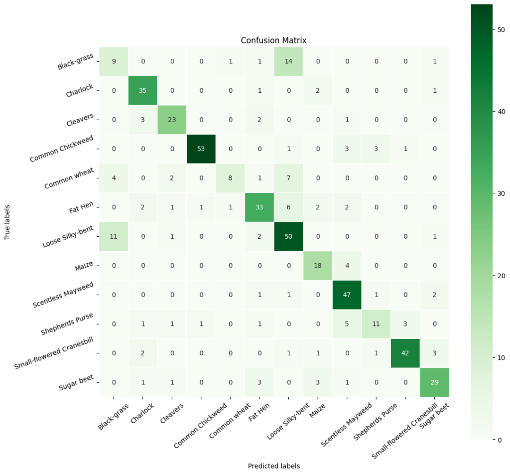
In [ ]:#Obtain categorical varaibles from y_test_encoded and y_pred y2_pred_arg = np.argmax(y2_pred, axis=1) y2_test_arg = np.argmax(y_test_encoded, axis=1) #Plotting confusion matrix confusion_matrix = tf.math.confusion_matrix(y2_test_arg, y2_pred_arg) f,ax = plt.subplots(figsize=(12,12)) sns.heatmap( confusion_matrix, annot=True, linewidths=0.4, fmt=‘d’, square=True, ax=ax, cmap=‘Greens’ # Set the colormap to Green ) #Setting labels to both axes ax.set_xlabel(‘Predicted labels’); ax.set_ylabel(‘True labels’); ax.set_title(‘Confusion Matrix’); ax.xaxis.set_ticklabels(list(enc.classes_),rotation=40) ax.yaxis.set_ticklabels(list(enc.classes_),rotation=20) plt.show()
In [ ]:# Calculate the classification report cr2 = metrics.classification_report(y2_test_arg, y2_pred_arg) # Print the classification report print(cr2) precision recall f1-score support 0 0.38 0.35 0.36 26 1 0.80 0.90 0.84 39 2 0.79 0.79 0.79 29 3 0.96 0.87 0.91 61 4 0.80 0.36 0.50 22 5 0.73 0.69 0.71 48 6 0.62 0.77 0.69 65 7 0.69 0.82 0.75 22 8 0.75 0.90 0.82 52 9 0.69 0.48 0.56 23 10 0.91 0.84 0.87 50 11 0.78 0.76 0.77 38 accuracy 0.75 475 macro avg 0.74 0.71 0.72 475 weighted avg 0.76 0.75 0.75 475
Observations:
- The revised model has an accuracy of 0.7537, which means that it correctly predicts the class labels for 75.37% of the instances in the dataset.
- The precision, recall, and F1-score vary for each class, indicating that the model’s performance is better for some classes (e.g., class 1) compared to others (e.g., class 0).
Final Model
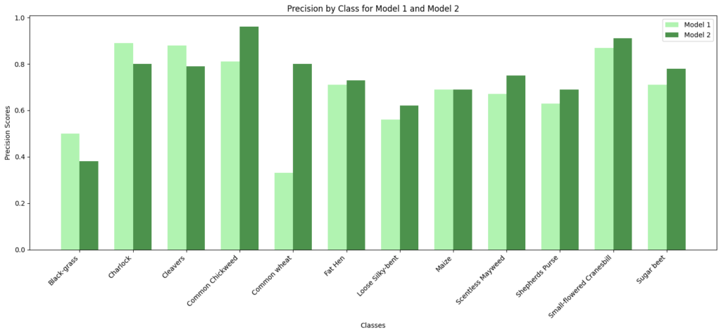
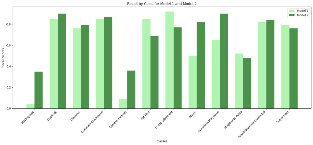
In [ ]:#Code to compare precision and recall scores of Model 1 vs Model 2# Class names class_names = np.unique(labels) model1_precision = [0.50, 0.89, 0.88, 0.81, 0.33, 0.71, 0.56, 0.69, 0.67, 0.63, 0.87, 0.71] model2_precision = [0.38, 0.80, 0.79, 0.96, 0.80, 0.73, 0.62, 0.69, 0.75, 0.69, 0.91, 0.78] model1_recall = [0.04, 0.85, 0.76, 0.85, 0.09, 0.85, 0.92, 0.50, 0.65, 0.52, 0.82, 0.79] model2_recall = [0.35, 0.90, 0.79, 0.87, 0.36, 0.69, 0.77, 0.82, 0.90, 0.48, 0.84, 0.76] # Set the width of the bars bar_width = 0.35 index = np.arange(len(class_names)) # Create subplots for precision fig, ax = plt.subplots() bar1 = ax.bar(index – bar_width/2, model1_precision, bar_width, label=‘Model 1’, color=‘lightgreen’, alpha=0.7) bar2 = ax.bar(index + bar_width/2, model2_precision, bar_width, label=‘Model 2’, color=‘darkgreen’, alpha=0.7) # Customize the plot for precision ax.set_xlabel(‘Classes’) ax.set_ylabel(‘Precision Scores’) ax.set_title(‘Precision by Class for Model 1 and Model 2’) ax.set_xticks(index) ax.set_xticklabels(class_names, rotation=45, ha=‘right’) ax.legend() # Display the precision plot plt.tight_layout() plt.show() # Create subplots for recall fig, ax = plt.subplots() bar1 = ax.bar(index – bar_width/2, model1_recall, bar_width, label=‘Model 1’, color=‘lightgreen’, alpha=0.7) bar2 = ax.bar(index + bar_width/2, model2_recall, bar_width, label=‘Model 2’, color=‘darkgreen’, alpha=0.7) # Customize the plot for recall ax.set_xlabel(‘Classes’) ax.set_ylabel(‘Recall Scores’) ax.set_title(‘Recall by Class for Model 1 and Model 2’) ax.set_xticks(index) ax.set_xticklabels(class_names, rotation=45, ha=‘right’) ax.legend() # Display the recall plot plt.tight_layout() plt.show()
Observations:
- Model 2’s performance is particularly strong in Charlock, Common Chickweed, Fat Hen, and Small-flowered Cranesbill, where it achieves high precision and recall scores.
- Class-Specific Performance: Model 2 generally outperforms Model 1 in terms of precision, recall, and F1-score for most classes. It has higher precision for many classes, meaning it is better at minimizing false positives. Model 1 has better recall for a few classes, but overall, Model 2 has better or similar recall.
- Model 2 has Higher Accuracy: Model 2 has a higher overall accuracy (0.75) compared to Model 1 (0.66), indicating that it makes more correct predictions on average.
Based on these observations, Model 2 is our choice for the final model.
Visualizing the prediction
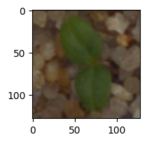
In [ ]:# Visualizing the predicted and correct label of images from test data# First image (index 2) plt.figure(figsize=(2, 2)) plt.imshow(X_test[2]) plt.show() # Complete the code to predict the test data using the final model selected predicted_label = model2.predict(X_test_normalized[2].reshape(1, 64, 64, 3)) predicted_label = enc.inverse_transform(predicted_label) true_label = enc.inverse_transform(y_test_encoded)[2] print(‘Predicted Label:’, predicted_label[0]) print(‘True Label:’, true_label) # Second image (index 33) plt.figure(figsize=(2, 2)) plt.imshow(X_test[33]) plt.show() # Complete the code to predict the test data using the final model selected predicted_label = model2.predict(X_test_normalized[33].reshape(1, 64, 64, 3)) predicted_label = enc.inverse_transform(predicted_label) true_label = enc.inverse_transform(y_test_encoded)[33] print(‘Predicted Label:’, predicted_label[0]) print(‘True Label:’, true_label) # Third image (index 59) plt.figure(figsize=(2, 2)) plt.imshow(X_test[59]) plt.show() # Complete the code to predict the test data using the final model selected predicted_label = model2.predict(X_test_normalized[59].reshape(1, 64, 64, 3)) predicted_label = enc.inverse_transform(predicted_label) true_label = enc.inverse_transform(y_test_encoded)[59] print(‘Predicted Label:’, predicted_label[0]) print(‘True Label:’, true_label) # Fourth image (index 36) plt.figure(figsize=(2, 2)) plt.imshow(X_test[36]) plt.show() # Complete the code to predict the test data using the final model selected predicted_label = model2.predict(X_test_normalized[36].reshape(1, 64, 64, 3)) predicted_label = enc.inverse_transform(predicted_label) true_label = enc.inverse_transform(y_test_encoded)[36] print(‘Predicted Label:’, predicted_label[0]) print(‘True Label:’, true_label)
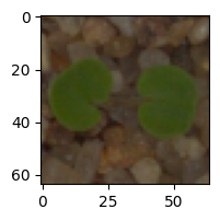
1/1 [==============================] – 0s 184ms/step Predicted Label: Small-flowered Cranesbill True Label: Small-flowered Cranesbill
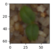
1/1 [==============================] – 0s 20ms/step Predicted Label: Cleavers True Label: Cleavers
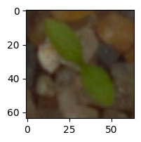
1/1 [==============================] – 0s 23ms/step Predicted Label: Common Chickweed True Label: Common Chickweed
1/1 [==============================] – 0s 18ms/step Predicted Label: Shepherds Purse True Label: Shepherds Purse
Recommendations and Insights
- With an accuracy of roughly 75% on test data, the model is able to significantly reduce the time and effort required to identify these plants. With additional data, the model can be tuned and likely achieve even better results.(We will explore pre-trained models to see if we could improve perfromance further. This would be in Appendix)
- This model could be integrated with automatic weeding systems, allowing weeds to be targeted over crops, reduce the amount of pesticides used overall, and lead to more eco-friendly farming.
APPENDIX:
Experimenting with pre trained models.
MobileNetV2
- MobileNetV2 is a lightweight convolutional neural network (CNN) architecture tailored for efficient image classification and object detection, especially on mobile and embedded devices.
- It builds upon the original MobileNet design, focusing on enhancing efficiency and maintaining high accuracy.
- MobileNetV2 typically consists of approximately 3.4 million parameters and is structured with multiple layers. Its architecture includes depth-wise separable convolutions and inverted residual blocks, with a variable number of these blocks depending on the specific model variant.
- This efficient design is a key strength of MobileNetV2, enabling powerful computer vision tasks with relatively few parameters, making it well-suited for resource-constrained environments.
- We will be using this model for our next level of model building.
In [ ]:#MobileNetv2 takes images in 128×128 or higher dimensions. So we are taking orignial dataset.#We are splitting the data set again.from sklearn.model_selection import train_test_split # Split the data into a temporary set and a test set X3_temp, X3_test, y3_temp, y3_test = train_test_split(np.array(images), labels, test_size=0.1, random_state=42, stratify=labels) # Split the temporary set into a training set and a validation set X3_train, X3_val, y3_train, y3_val = train_test_split(X3_temp, y3_temp, test_size=0.1, random_state=42, stratify=y3_temp)
In [ ]:print(X3_train.shape, y3_train.shape) # Check the shape of the training data and labels print(X3_val.shape, y3_val.shape) # Check the shape of the validation data and labels print(X3_test.shape, y3_test.shape) (3847, 128, 128, 3) (3847, 1) (428, 128, 128, 3) (428, 1) (475, 128, 128, 3) (475, 1)
In [ ]:#printing one of the orignial images plt.imshow(images[3])
Out[ ]:<matplotlib.image.AxesImage at 0x78f7b72962f0>

In [499]:#LabelBinarizer helps translate categories or labelsfrom sklearn.preprocessing import LabelBinarizer # Initialize the LabelBinarizer enc = LabelBinarizer() # Fit and transform y_train y3_train_encoded = enc.fit_transform(y3_train) # Transform y_val y3_val_encoded = enc.transform(y3_val) # Transform y_test y3_test_encoded = enc.transform(y3_test)
In [500]:#printing the shape of target train, encloded and test y3_train_encoded.shape, y3_val_encoded.shape, y3_test_encoded.shape
Out[500]:((3847, 12), (428, 12), (475, 12))
In [501]:#Code to normalize the image pixels of train, test and validation data X3_train_normalized = X3_train.astype(‘float32’) / 255.0 X3_val_normalized = X3_val.astype(‘float32’) / 255.0 X3_test_normalized = X3_test.astype(‘float32’) / 255.0
In [502]:#clearing backendfrom tensorflow.keras import backend backend.clear_session() #fixing random seed generatorsimport random np.random.seed(42) random.seed(42) tf.random.set_seed(42)
In [503]:from tensorflow.keras.models import Sequential from tensorflow.keras.layers import Dense, Dropout, GlobalAveragePooling2D from tensorflow.keras.applications import MobileNetV2 # Load MobileNetV2 Model without top base_model = MobileNetV2(weights=‘imagenet’, include_top=False, input_shape=(128, 128, 3)) # Freeze the layers of the base model base_model.trainable =False# Initializing the model model3 = Sequential() model3.add(base_model) model3.add(GlobalAveragePooling2D()) # Adding custom layers model3.add(Dense(32, activation=‘relu’)) # Output layer model3.add(Dense(12, activation=‘softmax’)) # Using softmax in output layers as we have 12 classes# Compile the model opt = Adam() model3.compile(optimizer=opt, loss=‘categorical_crossentropy’, metrics=[‘accuracy’]) # Display the model’s architecture model3.summary() Model: “sequential” _________________________________________________________________ Layer (type) Output Shape Param # ================================================================= mobilenetv2_1.00_128 (Func (None, 4, 4, 1280) 2257984 tional) global_average_pooling2d ( (None, 1280) 0 GlobalAveragePooling2D) dense (Dense) (None, 32) 40992 dense_1 (Dense) (None, 12) 396 ================================================================= Total params: 2299372 (8.77 MB) Trainable params: 41388 (161.67 KB) Non-trainable params: 2257984 (8.61 MB) _________________________________________________________________
In [506]:from tensorflow.keras.callbacks import EarlyStopping #Define EarlyStopping callback early_stopping = EarlyStopping( monitor=‘val_loss’, # Monitor validation loss patience=3, # Number of epochs with no improvement before stopping restore_best_weights=True# Restore the model weights to the best epoch ) # Train the model with EarlyStopping history_3 = model3.fit( X3_train_normalized, y3_train_encoded, epochs=12, batch_size=60, validation_data=(X3_val_normalized,y3_val_encoded), callbacks=[early_stopping] # Include the EarlyStopping callback ) Epoch 1/12 65/65 [==============================] – 8s 50ms/step – loss: 1.7020 – accuracy: 0.4432 – val_loss: 1.2138 – val_accuracy: 0.5911 Epoch 2/12 65/65 [==============================] – 2s 31ms/step – loss: 1.0019 – accuracy: 0.6743 – val_loss: 0.9319 – val_accuracy: 0.6846 Epoch 3/12 65/65 [==============================] – 2s 31ms/step – loss: 0.7734 – accuracy: 0.7458 – val_loss: 0.8262 – val_accuracy: 0.7103 Epoch 4/12 65/65 [==============================] – 2s 31ms/step – loss: 0.6380 – accuracy: 0.8001 – val_loss: 0.7619 – val_accuracy: 0.7570 Epoch 5/12 65/65 [==============================] – 2s 31ms/step – loss: 0.5504 – accuracy: 0.8271 – val_loss: 0.7210 – val_accuracy: 0.7710 Epoch 6/12 65/65 [==============================] – 2s 31ms/step – loss: 0.4813 – accuracy: 0.8503 – val_loss: 0.7080 – val_accuracy: 0.7944 Epoch 7/12 65/65 [==============================] – 2s 31ms/step – loss: 0.4269 – accuracy: 0.8721 – val_loss: 0.6937 – val_accuracy: 0.7687 Epoch 8/12 65/65 [==============================] – 2s 31ms/step – loss: 0.3882 – accuracy: 0.8893 – val_loss: 0.6552 – val_accuracy: 0.7874 Epoch 9/12 65/65 [==============================] – 2s 30ms/step – loss: 0.3421 – accuracy: 0.9002 – val_loss: 0.6714 – val_accuracy: 0.7780 Epoch 10/12 65/65 [==============================] – 2s 31ms/step – loss: 0.3240 – accuracy: 0.9038 – val_loss: 0.6509 – val_accuracy: 0.8014 Epoch 11/12 65/65 [==============================] – 2s 31ms/step – loss: 0.2855 – accuracy: 0.9212 – val_loss: 0.6491 – val_accuracy: 0.7921 Epoch 12/12 65/65 [==============================] – 2s 32ms/step – loss: 0.2644 – accuracy: 0.9244 – val_loss: 0.6487 – val_accuracy: 0.7991
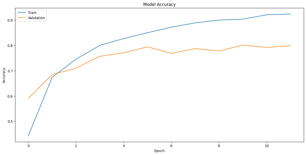
In [507]:plt.plot(history_3.history[‘accuracy’]) plt.plot(history_3.history[‘val_accuracy’]) plt.title(‘Model Accuracy’) plt.ylabel(‘Accuracy’) plt.xlabel(‘Epoch’) plt.legend([‘Train’,’Validation’], loc=‘upper left’) plt.show()
In [508]:#Evaluating the model on test data accuracy = model3.evaluate(X3_test_normalized, y3_test_encoded, verbose=2) 15/15 – 0s – loss: 0.6935 – accuracy: 0.7916 – 302ms/epoch – 20ms/step
In [509]:#Code to obtain the output probabilities y3_pred = model3.predict(X3_test_normalized) 15/15 [==============================] – 1s 20ms/step
Observations:
The model achieves an overall accuracy of 79.16% on the test set. This is a high accuracy rate, indicating that the model is robust and performs well across various classes of plant seedlings.
Plotting the Confusion Matrix
In [512]:# Obtaining the categorical values from y_test_encoded and y_pred y3_pred_arg=np.argmax(y3_pred,axis=1) y3_test_arg=np.argmax(y3_test_encoded,axis=1) # Plotting the Confusion Matrix using confusion matrix() function which is also predefined in tensorflow module confusion_matrix = tf.math.confusion_matrix(y3_test_arg, y3_pred_arg) # Complete the code to obatin the confusion matrix f, ax = plt.subplots(figsize=(12, 12)) sns.heatmap( confusion_matrix, annot=True, linewidths=.4, fmt=“d”, square=True, ax=ax, cmap=‘Greens’ ) # Setting the labels to both the axes ax.set_xlabel(‘Predicted labels’);ax.set_ylabel(‘True labels’); ax.set_title(‘Confusion Matrix’); ax.xaxis.set_ticklabels(list(enc.classes_),rotation=40) ax.yaxis.set_ticklabels(list(enc.classes_),rotation=20) plt.show()
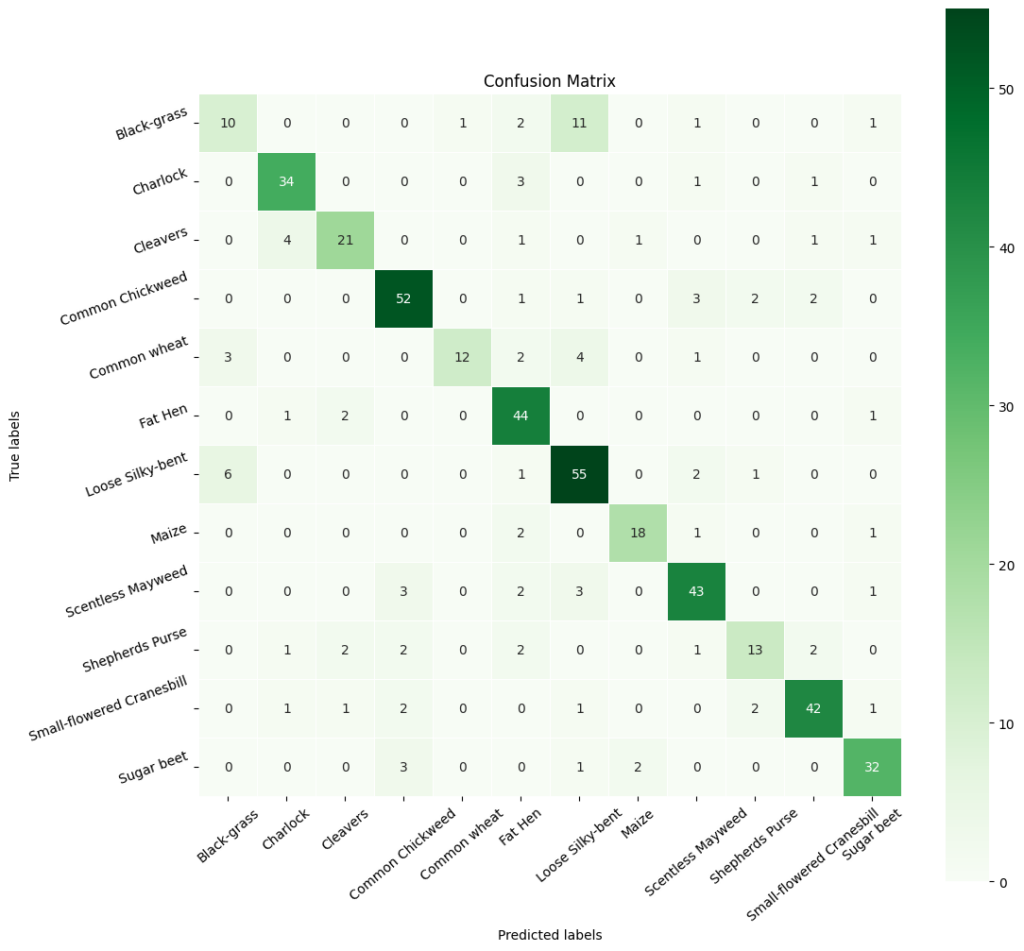
In [ ]:# Calculate the classification report cr3 = metrics.classification_report(y3_test_arg, y3_pred_arg) # Print the classification report print(cr3) precision recall f1-score support 0 0.56 0.38 0.45 26 1 0.81 0.87 0.84 39 2 0.82 0.79 0.81 29 3 0.88 0.84 0.86 61 4 0.93 0.59 0.72 22 5 0.75 0.88 0.81 48 6 0.72 0.86 0.78 65 7 0.89 0.77 0.83 22 8 0.77 0.85 0.81 52 9 0.65 0.48 0.55 23 10 0.86 0.86 0.86 50 11 0.87 0.87 0.87 38 accuracy 0.79 475 macro avg 0.79 0.75 0.77 475 weighted avg 0.79 0.79 0.79 475
Precision, Recall, and F1-Scores:
The precision across classes is mostly high, with ‘Common Chickweed’ (label 3),’Common wheat'(label4), ‘Maize’ (label 7),’Sugar beet'(label 10), and 11’Charlock’ showing particularly strong precision of 0.85 or above. This indicates that when the model predicts these classes, it is very likely to be correct.
The recall is also notably high for most classes, with ‘Sugar beet’, ‘Charlock’ and ‘Common Chickweed’ again standing out, suggesting that the model is capable of identifying most of the true positives for these classes.
The F1-scores, which are the harmonic mean of precision and recall, are uniformly high across most classes, indicating that the model maintains a good balance between the precision and recall. This balance is crucial in practical applications where both identifying the correct class and minimizing false positives are important.
Class-Specific Performance:
While most classes exhibit strong F1-scores, the class ‘Black-grass’ (label 0) has a lower F1-score of 0.56 (but best across models). This suggests that there may be characteristics of this class that are not being captured as effectively as others, which may be due to intra-class variability or similarities with other classes. The class ‘Small-flowered Cranesbill’ (label 4) also shows a slightly lower recall and F1-score compared to its precision, indicating that while the model is highly confident when it predicts this class, it is missing some true positives.
Model Consistency:
The training and validation accuracy curves show a consistent improvement over epochs, with the training accuracy reaching a high level. This suggests that the model is learning effectively from the training data. The validation accuracy curve is smooth and does not exhibit high variance, which would indicate overfitting. This suggests that the model generalizes well to unseen data.
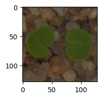
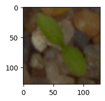
In [ ]:# Visualizing the predicted and correct label of images from test data# First image (index 2) plt.figure(figsize=(2, 2)) plt.imshow(X3_test[2]) plt.show() # Complete the code to predict the test data using the final model selected predicted_label = model3.predict(X3_test_normalized[2].reshape(1, 128, 128, 3)) predicted_label = enc.inverse_transform(predicted_label) true_label = enc.inverse_transform(y3_test_encoded)[2] print(‘Predicted Label:’, predicted_label[0]) print(‘True Label:’, true_label) # Second image (index 33) plt.figure(figsize=(2, 2)) plt.imshow(X3_test[33]) plt.show() # Complete the code to predict the test data using the final model selected predicted_label = model3.predict(X3_test_normalized[33].reshape(1, 128, 128, 3)) predicted_label = enc.inverse_transform(predicted_label) true_label = enc.inverse_transform(y3_test_encoded)[33] print(‘Predicted Label:’, predicted_label[0]) print(‘True Label:’, true_label) # Third image (index 59) plt.figure(figsize=(2, 2)) plt.imshow(X3_test[59]) plt.show() # Complete the code to predict the test data using the final model selected predicted_label = model3.predict(X3_test_normalized[59].reshape(1, 128, 128, 3)) predicted_label = enc.inverse_transform(predicted_label) true_label = enc.inverse_transform(y3_test_encoded)[59] print(‘Predicted Label:’, predicted_label[0]) print(‘True Label:’, true_label) # Fourth image (index 37) plt.figure(figsize=(2, 2)) plt.imshow(X3_test[37]) plt.show() # Code to predict the test data using the final model selected predicted_label = model3.predict(X3_test_normalized[37].reshape(1, 128, 128, 3)) predicted_label = enc.inverse_transform(predicted_label) true_label = enc.inverse_transform(y3_test_encoded)[37] print(‘Predicted Label:’, predicted_label[0]) print(‘True Label:’, true_label)
1/1 [==============================] – 0s 22ms/step Predicted Label: Small-flowered Cranesbill True Label: Small-flowered Cranesbill
1/1 [==============================] – 0s 22ms/step Predicted Label: Cleavers True Label: Cleavers
1/1 [==============================] – 0s 22ms/step Predicted Label: Common Chickweed True Label: Common Chickweed
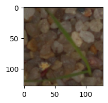
1/1 [==============================] – 0s 26ms/step Predicted Label: Loose Silky-bent True Label: Loose Silky-bent
Business Insights
- By using a pre-trained model, MobileNetV2, we were able to improve the accuracy of the model from our best score of 75% on test data to 79.3%.
- The recall and F1 score has improved for most classes.
- The improved accuracy of Model 3 using MobileNet demonstrates the potential for deploying deep learning models in agricultural settings. The ability to accurately classify plant species can enhance crop management and weed control practices.
Recommendations
- Model Deployment: With an accuracy of 79.3% and high F1-scores for most classes, the model is approaching a level of reliability suitable for real-world application, which could significantly reduce the time and labor costs associated with manual plant sorting.
- Expert Collaboration: Work with agricultural scientists to understand the nuances of different species and to identify any additional features that could be used to improve model accuracy. This domain expertise can guide further feature engineering and data collection efforts.
- Educational Programs: Educate the end-users, such as farmers and agricultural workers, on how to use the technology effectively. Offer workshops or training sessions to ensure they can leverage the AI system to its full potential.
By adopting these recommendations, the agricultural business can leverage AI to enhance productivity, reduce costs, and support sustainable farming practices. The long-term goal should be not only to implement current models but also to foster an environment of continuous improvement and adaptation to technological advancements in AI and machine learning.